Principal Component Analysis
Table of contents
0. (Multiple) Linear Regression by LSE
\[\hat{y} = X\hat{\theta}\](1) model
\[\mathbf{y} = X\mathbf{\theta} + \mathbf{\epsilon}\](2) notation
- $(X\vert\mathbf{y})$ : dataset
- $n+1$ : dimension of regression (with bias $\theta_0$)
- $m$ : the number of data
- $\mathbf{y}_{m \times 1}$ : target data (vector)
- $X_{m \times (n+1)}$ : feature data (matrix)
- $\mathbf{\theta}_{(n+1) \times 1}$ : parameter (vector)
- $\hat{(\cdot)}$ : estimate of $(\cdot)$
(2) problem
\[\min\limits_{\theta}S(\theta) = \sum\limits_{1\le j \le m} \epsilon_j^2\]$S(\mathbf{\theta})$ : square sum of errors of each data
(3) solution
\[X^TX\hat{\mathbf{\theta}} = X^T\mathbf{y}\](4) geometric interpretation of error $\mathbf{\epsilon}$
basis direction distance from target data $\mathbf{y}$ to regression hyperplain $\mathbf{x}^T\mathbf{\theta}$
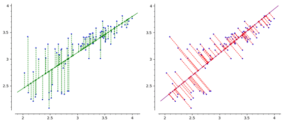 |
|---|
| (left) LSE / (right) PCA |
1. PCA (to 1-dim)
(1) geometric interpretation
\[\min\limits_{\overrightarrow{\mathbf{e}}} d(\overrightarrow{\mathbf{e}})\]$d(\overrightarrow{\mathbf{e}})$ : distance from target data $\mathbf{y}$ to orthogonal projection onto an 1-d line with unit direction vector $\overrightarrow{\mathbf{e}}$
(2) solution
\[\overrightarrow{\mathbf{e}} = \mathbf{u}_1\]$\mathbf{u}_1$ : the 1st singular vector of centralized dataset $X$
(3) proof
Let $P = \mathbf{e}\mathbf{e}^T$. Then $P^2 = P = P^T$ since $\mathbf{e}$ is a unit.
Thus $P$ is an orthogonal projection matrix onto $C(P) = \text{span}(\mathbf{\lbrace e\rbrace })$.
$\mathbf{x}_i$ : $i$ th data ($i$ th row of $X$)
\[\begin{align*} \lVert\mathbf{x} - P\mathbf{x}_i\rVert &= \lVert(I-P)\mathbf{x}\rVert \\ &= \mathbf{x}^T(I-P)^T(I-P)\mathbf{x} \\ &= \mathbf{x}^T(I-P^T-P+P^TP)\mathbf{x} \\ &= \mathbf{x}^T(I-P)\mathbf{x} \ (\because P^2=P=P^T) \\ &= \mathbf{x}^T\mathbf{x} - \mathbf{x}^T\mathbf{e}\mathbf{e}^T\mathbf{x} \ (\because P=\mathbf{e}\mathbf{e}^T) \end{align*}\]Thus,
\[\begin{align*} d(\mathbf{e}) &= \sum_{i=1}^{m} \lVert \mathbf{x}_i-P\mathbf{x}_i \rVert \\ &= \sum_{i=1}^{m}(\mathbf{x}_i^T\mathbf{x}_i-\mathbf{x}_i^T\mathbf{e}\mathbf{e}^T\mathbf{x}_i) \\ &= \sum_{i=1}^{m}\mathbf{x}_i^T\mathbf{x}_i - \sum_{i=1}^{m} (\mathbf{x}_i^T\mathbf{e})^2 \ (\because \mathbf{x}_i^T\mathbf{e} = \mathbf{e}^T\mathbf{x}_i \text{ : scalar}) \\ &= \sum_{i=1}^{m}\mathbf{x}_i^T\mathbf{x}_i - \lVert X\mathbf{e} \rVert \\ &= \sum_{i=1}^{m}\mathbf{x}_i^T\mathbf{x}_i - \mathbf{e}^TX^T X\mathbf{e} \end{align*}\]Thus,
\[\min\limits_{\lVert\mathbf{e}\rVert=1}d(\mathbf{e}) \iff \max\limits_{\lVert\mathbf{e}\rVert=1} (\mathbf{e}^TX^T X\mathbf{e})\]Let Lagrange $ \mathscr{L}(\mathbf{e}) = \mathbf{e}^TX^TX\mathbf{e} - \lambda(\left\lvert\mathbf{e}\right\rvert^2-1) $
From $\dfrac{\partial \mathscr{L}}{\partial \mathbf{e}} = 2X^TX\mathbf{e}-2\lambda\mathbf{e} = 0$, we obtain $X^TX\mathbf{e} = \lambda\mathbf{e}$.
Then,
Hence
\[\begin{align*} \mathop{\text{argmin}}\limits_{\lVert\mathbf{e}\rVert=1}d(\mathbf{e}) &= \text{eigenvector of } X^TX \text{ (corresponding to the largest eigenvalue)} \\ &= \text{1st right singular vector } \mathbf{v}_1 \text{ of } X = U\Sigma V^T \end{align*}\]이때 singular vector $\mathbf{v}_1$ 을 주성분이라 한다.
일반화하여 $n$-dimension $(n \ge 2)$ 으로 차원축소하는 경우, leading singular vectors 들이 주성분이 된다.
(4) Statistical View
Assume that dataset $X$ is centralized. ($X \leftarrow X- \underset{col}{E}(X)$)
Let $V=\dfrac{1}{m-1}X^TX$, then $V$ is the (sample) covariance matrix of dataset since for $V=(v_{ij})_{(n+1)\times(n+1)}$,
For each data $\mathbf{x}_i$,
\[(\text{projection onto }\mathbf{e}) = (\mathbf{x}_i^T\mathbf{e})\mathbf{e}\]Thus
\[\begin{align*} \text{Var}(\lVert(X\mathbf{e})\mathbf{e}\rVert) &= \text{Var}(X\mathbf{e}) \\ &= \frac{1}{m-1}\mathbf{e}^TX^TX\mathbf{e} \\ &= \mathbf{e}^TV\mathbf{e} \end{align*}\]Thus,
\[\begin{align*} \min\limits_{\lVert\mathbf{e}\rVert=1}d(\mathbf{e}) &\iff \max\limits_{\lVert\mathbf{e}\rVert=1} \mathbf{e}^TV\mathbf{e} \\ &\iff \max\limits_{\lVert\mathbf{e}\rVert=1} \text{Var}( \ \lVert \text{data projection onto }\mathbf{e}\rVert \ ) \end{align*}\]결과적으로 데이터의 분산을 최대로 보존하는 방향으로 projection 을 함으로써, 차원을 축소하면서도 정보 손실을 최소화(MSE를 기준으로)한다.