Logistic Regression
Table of contents
- 0. sigmoid / softmax function
- 1. model
- 2. Decision Boundary
- 3. Loss Function
- 4. gradient descent : probabilistic setting
Linear Classifier by affine transformation
0. sigmoid / softmax function
- odds : $(0, 1) \rightarrow (0, \infty)$
- logit transformation : $(0, 1) \rightarrow (-\infty, \infty)$
- sigmoid function (inverse of logit) : $(-\infty, \infty) \rightarrow (0, 1)$
- softmax function (generalized sigmoid) : $(-\infty, \infty)^n \rightarrow (0, 1)^n$
If $n=2$ (binary, sigmoid)
\[\bm\sigma({\mathbf{x}})_1 = \frac{e^{x_1}}{e^{x_1} + e^{x_2}} = \frac{1}{1 + e^{x_2 - x_1}} = \sigma(x_2 - x_1)\]thus domain of sigmoid function can be interpreted as the score difference.
1. model
binary classification
\[P(y = 1 \vert \mathbf{x}) = \sigma(\mathbf{w}^T \mathbf{x}) = \frac{1}{1 + e^{w_0 + w_1 x_1 + \cdots + w_k x_k}}\]multiple classification
\[P(y = c_i \vert \mathbf{x}) = \bm\sigma(W \mathbf{x})_i = \frac{e^{\mathbf{w}_i^T \mathbf{x}}}{e^{\mathbf{w}_1^T \mathbf{x}} + e^{\mathbf{w}_2^T \mathbf{x}} + \cdots + e^{\mathbf{w}_k^T \mathbf{x}}} , \quad W = \begin{bmatrix} \mathbf{w}_1^T \\ \mathbf{w}_2^T \\ \vdots \\ \mathbf{w}_k^T \end{bmatrix}\]Each $\mathbf{w}_i^T \mathbf{x}$ can be interpreted as the i-th class score.
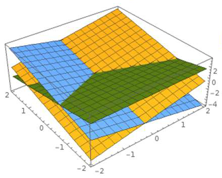
2. Decision Boundary
Assume that a data point $\mathbf{x}$ is classified as the i-th class if the score $P(y = c_i \vert \mathbf{x}) > p $ for some $p \in (0, 1)$.
Then
\[P(y = c_i \vert \mathbf{x}) > p \iff \mathbf{w}_i^T \mathbf{x} > c\]where $ c = \text{ln}[p(e^{\mathbf{w}_1^T \mathbf{x}} + e^{\mathbf{w}_2^T \mathbf{x}} + \cdots + e^{\mathbf{w}_k^T \mathbf{x}})]$
A hyperplain $ \mathbf{w}_i^T \mathbf{x} = c $ is called decision boundary.
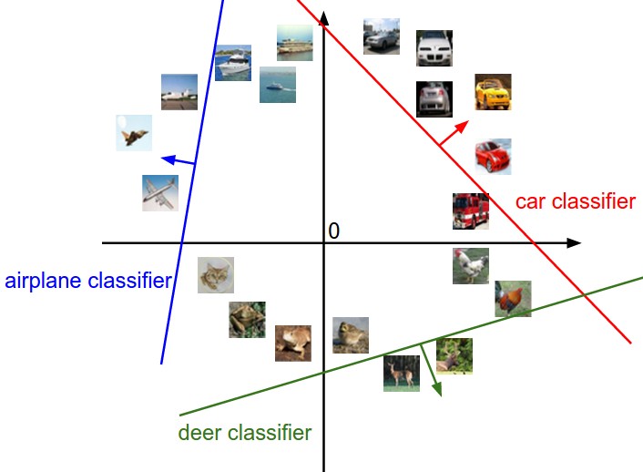 |  |
|---|---|
| decision boundary - threshold classification | decision boundary - max classification |
3. Loss Function
(1) discriminative setting (binary classification)
- ground truth $y \in \lbrace +1, -1 \rbrace $
- predicted score $\hat{y} \in \mathbb{R}$
- margin $y \hat{y}$
margin-based loss function
| 0/1 loss | log loss | exponential loss | hinge loss |
|---|---|---|---|
| $I_{(y\hat{y}<0)}$ | $\text{log}(1 + e^{-y \hat{y}})$ | $e^{-y \hat{y}}$ | $\text{max}\lbrace 0, 1- y \hat{y} \rbrace$ |
| not continuous not diff’able at $y \hat{y}=0$ | interpretable $p(y \vert x)$ (logistic regression) | vulnerable to outliers | computationally efficient (SVM) |
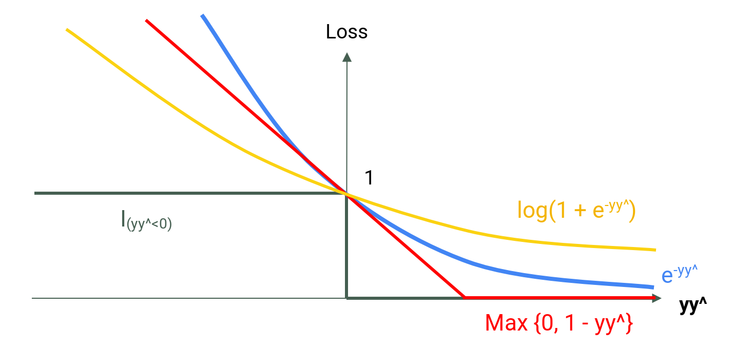 |
|---|
| a rough form of graphs |
more margin-based loss function - GitHub blog
(2) probabilistic setting
- ground truth $y \in \lbrace 0, 1 \rbrace $ for a binary classification
- ground truth $\mathbf{y} = (y_k) \in \lbrace 0, 1 \rbrace ^K$ : an one-hot vector for a multi-class classification
- predicted score $\hat{\mathbf{y}} \in [0,1]^K$
- compare two probability distribution, our model and the empirical distribution
information theory
where
$m$ : number of data,
$K$ : number of classes, and
$\hat{y}_{iT_i}$ : predicted probability for the correct class (the degree of certainty).
Interpreting $\dfrac{1}{m}$ as a probability in the empirical distribution $P$,
\[\mathcal{L} = H(P, \hat{P})\]for our model (estimated distribution) $\hat{P}$.
4. gradient descent : probabilistic setting
(1) binary classification - sigmoid
\[\mathcal{L} = - \frac{1}{m} \sum_{i=1}^{m} \Big[ y_i \text{log}(\hat{y}_i) + (1-y_i) \text{log}(1 - \hat{y}_i) \Big]\]where $\hat{y}_i = \sigma(\mathbf{w}^T\mathbf{x}_i) := \sigma(z_i)$.
step-by-step
Note that $\sigma^\prime(x) = \sigma(x) \big( 1 - \sigma(x) \big)$. Let $$ \begin{align*} l_0(\mathbf{w}) &= (1-y_i) \text{log}(1 - \hat{y}_i) \\ &= (1-y_i) \text{log} \big( 1 - \sigma(\mathbf{w}^T\mathbf{x}_i) \big) \\ \\ l_1(\mathbf{w}) &= y_i \text{log}(\hat{y}_i) \\ &= y_i \text{log} \big( \sigma(\mathbf{w}^T\mathbf{x}_i) \big) \end{align*} $$ Then, $$ \begin{align*} \frac{\partial l_0(\mathbf{w})}{\partial w_j} &= (1 - y_i) \frac{1}{1-\sigma(z_i)} \Big[ -\sigma(z_i) \big( 1-\sigma(z_i) \big) \Big] \frac{\partial \mathbf{w}^T \mathbf{x}_i}{\partial w_j} \\ &= - (1-y_i) \sigma(z_i) x_{ij} \\ \\ \frac{\partial l_1(\mathbf{w})}{\partial w_j} &= y_i \frac{1}{\sigma(z_i)} \Big[ \sigma(z_i) \big( 1-\sigma(z_i) \big) \Big] \frac{\partial \mathbf{w}^T \mathbf{x}_i}{\partial w_j} \\ &= y_i \big( 1-\sigma(z_i) \big) x_{ij} \\ \\ \frac{\partial l_0(\mathbf{w})}{\partial w_j} + \frac{\partial l_1(\mathbf{w})}{\partial w_j} &= - x_{ij} \big( \sigma(z_i) - y_i \big) \\ &= - x_{ij} \big( \hat{y}_i - y_i \big) \end{align*} $$ Therefore, $$ \begin{align*} \frac{\partial \mathcal{L}}{\partial w_j} &= \frac{1}{m} \sum_{i=1}^{m} x_{ij} \big( \sigma(z_i) - y_i \big) \\ &= \frac{1}{m} \begin{bmatrix} x_{1j} \\ x_{2j} \\ \vdots \\ x_{mj} \end{bmatrix}^T (\hat{\mathbf{y}} - \mathbf{y}) \end{align*} $$ Note that $ \begin{bmatrix} x_{1j} \\ x_{2j} \\ \vdots \\ x_{mj} \end{bmatrix} $ is the *j*-th column of the feature matrix $X$. Hence,We obtain
\[\mathbf{w} \leftarrow \mathbf{w} - \alpha \cdot \frac{1}{m} X^T (\hat{\mathbf{y}} - \mathbf{y})\]This is the same result as in the case of a linear regression.
(2) multi-class classification - softmax : multinomial logistic regression
\[\mathcal{L} = - \frac{1}{m} \sum_{i=1}^{m} \sum_{k=1}^K y_{ik} \text{log}( \hat{y}_{ik} ) = - \frac{1}{m} \sum_{i=1}^m \text{log} ( \hat{y}_{iT_i})\]where $\hat{y}_{ik} = \bm\sigma (W\mathbf{x}_i)_k := \bm\sigma (\mathbf{z}_i)_k$.
Note that
\[X \overset{W}{\longrightarrow} \mathbf{z}_i \overset{\bm\sigma}{\longrightarrow} \mathbf{a} \overset{}{\longrightarrow} \mathcal{L}(W; \mathbf{x_i})\]notation
where $$ \begin{align*} X &=\begin{bmatrix} \mathbf{x}_1^T \\ \mathbf{x}_2^T \\ \vdots \\ \mathbf{x}_m^T \end{bmatrix} &&= \begin{bmatrix} 1 & x_{11} & x_{12} & \cdots & x_{1n} \\ 1 & x_{21} & x_{22} & \cdots & x_{2n} \\ \vdots & \vdots & \vdots & \ddots & \vdots \\ 1 & x_{m1} & x_{m2} & \cdots & x_{mn} \\ \end{bmatrix} \\ W &=\begin{bmatrix} \mathbf{w}_1^T \\ \mathbf{w}_2^T \\ \vdots \\ \mathbf{w}_K^T \end{bmatrix} &&= \begin{bmatrix} w_{10} & w_{11} & w_{12} & \cdots & w_{1n} \\ w_{20} & w_{21} & w_{22} & \cdots & w_{2n} \\ \vdots & \vdots & \vdots & \ddots & \vdots \\ w_{K0} & w_{K1} & w_{K2} & \cdots & w_{Kn} \\ \end{bmatrix} \\ \mathbf{z}_i &= W \mathbf{x}_i &&= \begin{bmatrix} \mathbf{w}_1^T \mathbf{x}_i \\ \mathbf{w}_2^T \mathbf{x}_i \\ \vdots \\ \mathbf{w}_K^T \mathbf{x}_i \end{bmatrix} \\ \quad \mathbf{a} &= \bm\sigma(\mathbf{z}_i) = \hat{\mathbf{y}}_i &&= \begin{bmatrix} \hat{y}_{i1} \\ \hat{y}_{i2} \\ \vdots \\ \hat{y}_{iK} \end{bmatrix} \\ \quad \mathcal{L}(W; \mathbf{x_i}) &= \mathcal{L} &&= - \frac{1}{m} \sum_{i=1}^m \mathbf{y}_i^T \text{log} ( \mathbf{a} ) \end{align*} $$This is just like backpropagation in neural network. So I omit the explanation in this post.